
In the Aerial Geodesy course of our school of quadcopter drone pilots, questions often arise related to coordination systems. This is a rather complicated topic for those who decide to become a drone pilot and master aerial geodesy without a basic geodetic education. We decided to fill this gap, and to optimize the learning process, we have presented here the material for self-study and use in the process of conducting aerial surveying with drones. This manual for training quadcopter pilots involved in aerial surveying provides a detailed description of the 1942 Coordinate System (SC-42), the most commonly used mapping coordinate system in the CIS countries. Some of the most important issues of geographic referencing of spatial data for users of geographic information systems are also considered.
Introduction
If you've ever held a sheet of topographic map (at a scale no smaller than 1:200,000) in your hands, you may have noticed the modest inscription in the upper left corner of the sheet, "1942 coordinate system."
The fact is that almost all large-scale topographic maps of the territory of the former USSR are made in this coordinate system. Most thematic maps, including geological maps, are also drawn in the 1942 coordinate system, as topographic maps were the basis for their creation. Geologists and geophysicists, working in the field or compiling reports, use topographic and other maps they are familiar with from year to year. However, few of them can clearly explain what the 1942 coordinate system is. Maybe they don't need to, if they have been working with paper maps all their lives. But for those who want to learn how to use a drone to survey and work with GIS, it is imperative to understand this issue.
The cartographic coordinate system of 1942 (SK-42) is a system of flat rectangular coordinates. It is based on the Gauss-Kruger projection, which was proposed in the first half of the XIX century and is still in use today. Often, the SK-42 and the Gauss-Kruger projection are identified, although, strictly speaking, they are not the same thing.
The process of transferring the real earth's surface to the map plane is a rather complicated and intricate path that is performed in several steps:
- The irregular shape of the Earth (geoid) is approximated by some regular surface (i.e., one that can be described by a single formula). The selected surface is fixed relative to the Earth's body and becomes the surface of reference (also called the reference surface). This defines the (geographic) coordinate system. The relativity surface is scaled according to the main map scale.
- The image of geographical objects from the surface of the belonging is displayed (projected) on a plane or a surface that can be deployed without distortion using strict mathematical methods.
Let's look at all these steps in turn.
1. Some concepts of the theory of the Earth's shape.
Even if you flew your quadcopter drone high enough during your training flights, you could not directly see the curvature of the Earth's surface. The theory of the Earth's shape uses the concept of a flat surface, which is defined as a continuous surface at all points in the normal direction of straight lines (the direction of gravity).
Obviously, you can imagine many flat surfaces that surround the Earth. The surface of the world's oceans at rest is also a flat surface. It is called the mean sea level surface, or geoid surface.
The surface of a geoid is not stable and, undergoing continuous changes over time, can only be recorded for a certain moment. Surface changes (fluctuations in the level of the world's oceans and land) are caused by the lunar-solar attraction that causes sea tides and various geological and meteorological factors, the mathematical description of which is difficult and often impossible. Therefore, fixing the surface of a geoid can only be done approximately, based on the results of long-term observation of the ocean level. In Russia, the zero of the Kronstadt footstock, which fixes the average level of the Baltic Sea, is taken as the starting point on the geoid surface.
The use of a geoid as a characteristic of the Earth's shape is complicated by the fact that to study the surface of a geoid, it is not enough to know the Earth's gravitational field, but it is necessary to use data on the density distribution of the Earth's crustal masses. The structure of the Earth's crust is not yet fully understood, and this makes it impossible to accurately determine the surface of the geoid and forces us to solve this problem approximately, resorting to certain hypotheses and assumptions.
Currently, a so-called quasi-geoid is used to study the shape of the Earth, as well as to solve geodetic problems (Fig. 1). The advantage of a quasi-geoid is that its surface can be studied only on the basis of gravimetric data, without involving data on the structure of the Earth's crust. Drones also help to cope with this task.
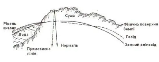
The surfaces of a geoid and a quasi-geoid coincide in the oceans, differ by no more than a few cm on the plains, and in mountainous areas the difference reaches 2 m (Fig. 1).
The surfaces of a geoid and quasi-geoid are not mathematically correct and unchanging in time, and therefore a stable and simpler comparison surface must be used to process geodetic measurements. In cartography, the surface of the ellipsoid of rotation is used as such.
Here we are forced to make a small digression from the general story for those who have no idea what an ellipsoid of rotation is and how they can represent the Earth's surface.
1.1 The concept of ellipsoidal rotations.
Just as a sphere is based on a circle, an ellipsoid is based on an ellipse. In general, we consider a three-axis ellipsoid. Depending on the ratio of the lengths of its axes, there are three possible cases: a sphere (all three axes are equal), an ellipsoid of rotation (two axes are equal), and a three-axis ellipsoid (all axes are different).
The sphere is used only for small-scale maps (smaller than 1:1000000). At these scales, it is impossible to tell the difference between a sphere and an ellipsoid on the map. However, to maintain the accuracy of larger scale maps, the Earth should be treated as an ellipsoid.
The three-axis ellipsoid is used almost exclusively to represent irregularly shaped celestial bodies. It is not relevant for representing the earth's surface in GIS, and is used only in particularly precise geodetic measurements. For the construction of topographic maps, the ellipsoid of rotation is chosen in most cases. Just as the rotation of a circle around an axis defined by its diameter forms a sphere, the rotation of an ellipse around its major or minor axis forms an ellipsoid.
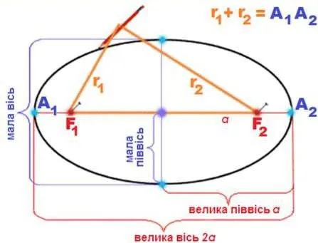
The ellipse is defined by two parameters - the length of the two semi-axes a and b (Fig. 2), or (more commonly) the length of the large semi-axis and the compression ratio f = (ab)/a . Compression values range from 0 to 1. A compression of 0 means that both axes are equal, i.e. we are dealing with a circle. A compression of 1 means a figure with only one axis, which looks like a line segment whose length is equal to the length of the major axis. In general, large compression values describe narrow ellipses, and small compression values describe almost circular ellipses.
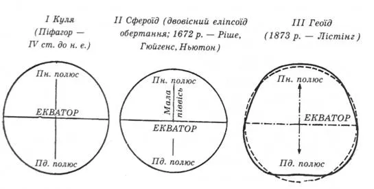
An ellipsoid that almost resembles a sphere is called a "spheroid" (Fig. 3). An ellipsoid that almost resembles the shape of the Earth is formed by rotation about a minor axis. The ellipticity of the sphere is 0, while the ellipticity of the Earth is approximately 0.003353. The phenomenon of compression is observed at the poles, while expansion occurs at the equator. Therefore, the major axis describes the equatorial radius, and the minor axis represents the polar radius.
The size of the ellipsoid and its orientation in the Earth's body should be such that the surfaces of the ellipsoid and quasi-geoid are as close to each other as possible. This is best satisfied by the World ellipsoid, which has
1) the center coincides with the center of gravity of the Earth, and the plane of the equator coincides with the plane of the Earth's equator,
2) the sum of the squares of deviations in height of the ellipsoid surface from the surface of the quasi-geoid is minimal.
Currently, the task of determining the parameters of the Earth's ellipsoid is solved by making measurements using satellite geodetic systems. The use of satellite technology has made it possible to identify several elliptical deviations: for example, the south pole is closer to the equator than the north pole. The general earth ellipsoid approximates the surface of the Earth as a whole. In the United States, the WGS-84 (World Geodetic System 1984) ellipsoid is currently used, and in the CIS - EO-90 (Earth Parameters 1990). The tasks of determining the size of the Earth's ellipsoid and its orientation in the Earth's body should be solved jointly. However, the exact fulfillment of the above conditions is impossible without a detailed study of the surface of the quasi-geoid as a whole.
Before the creation of satellite geodetic systems, ellipsoid parameters were determined as a result of computational processing of data from state and regional geodetic networks. In this case, the task of establishing an ellipsoid is usually divided into two parts: first, using the results of geodetic and gravimetric works, the dimensions of the ellipsoid are determined, and then the ellipsoid is oriented in the Earth. The ellipsoid obtained in this way is called a reference ellipsoid.
Since geodetic networks were created on different continents, with different means and with different levels of accuracy, there are currently more than two dozen reference ellipsoids, each of which is optimal only for a certain part of the Earth. For the territory of Russia, such an ellipsoid is the Krasovsky ellipsoid, calculated in 1940.
Thus, there are 2 types of ellipsoids: general ellipsoids that approximate the Earth's surface as a whole and reference ellipsoids that most accurately represent the Earth's surface in a limited area, for example, within a single country.
It should be noted that in the reference calculations, spheroids determined by satellite technology are beginning to replace spheroids determined by ground-based measurements.
A fact that must be taken into account before making changes to a reference spheroid is the effect of such a change on all previously measured values. Due to the difficulty of measuring spheroids, those that were derived from ground measurements are still in use and still provide valuable reference material. The names of some spheroids, axis sizes, and geographic locations to which they can be applied are listed in Table 1. You will notice that the values do vary, but only in small amounts relative to the size of the Earth.
Large and small spheroid semi-axes
2. Geodetic coordinate system (DATUM).
The next step is to set the geodetic coordinate system on the surface of the ellipsoid. The coordinates used are curvilinear coordinates known as latitude and longitude. Although the origin is defined as a point at the intersection of the equator and the Greenwich Meridian, in reality, an indirect method is used to set the coordinate reference, when the latitude and longitude values are fixed for a certain point on the real surface of the Earth (the so-called starting point), the normal to the surface of the reference ellipsoid and the straight line at this point are combined, and the plane of the starting point meridian is set parallel to the Earth's rotation axis. These initial data, also called geodetic dates (datum), rigidly fix the geodetic coordinate system relative to the Earth's body. For the Krasovsky ellipsoid, such a point is set in Pulkovo (the center of the observatory's round hall), and this sets the basis for the 1942 Coordinate System (CK-42).
3. Main and relative scales.
The design process can be simplified in 2 stages: first, we transform the Earth into an intermediate spheroid depending on the chosen scale, then this spheroid is projected onto a flat surface. The numerical scale of the first transformation is called the main scale: it is equal to the ratio of the radius of the intermediate spheroid to the radius of the Earth.
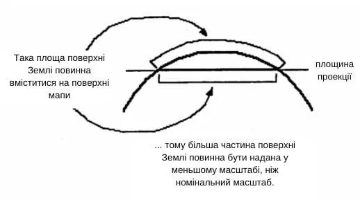
Now let's look at another new concept - the scale factor. The scale factor, also called relative scale, is defined as the ratio of the local scale on the map to the main scale. By definition, the scale factor on an intermediate spheroid is 1. When we move from its spherical surface to a plane with two axes, the local scale will not be equal to the main scale, since the flat and spherical surfaces are not compatible (Fig. 4). Therefore, the scale factor is generally not equal to 1 and will be different in different parts of the map. The more the scale factor differs from 1, the more distortion is present on the map.
4. 4. Cartographic projections.
A globe is a traditional way of showing the shape of the Earth. Although globes generally represent the shape of the Earth and show the spatial outlines of objects as large as a continent, they are not used in practice. Even a very small scale globe (1: 1000000000) will be very large, so you can't put it in your pocket and you can't plot a route for a drone on it. In practice, we use much larger scales to conduct fieldwork and analyze the data, anywhere from 1:1000000 to 1:5000, depending on the level of detail. Only a giantomaniac would dream of making a globe of this scale. Therefore, cartographers have developed a set of methods called cartographic projections, which are designed to depict the spherical Earth with acceptable accuracy on a flat medium.
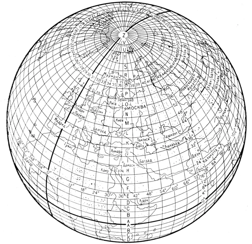
There is another reason why we use flat maps in practice. On a globe, it is quite easy to determine the location of an object, knowing its spherical latitude and longitude coordinates (Figure 5).
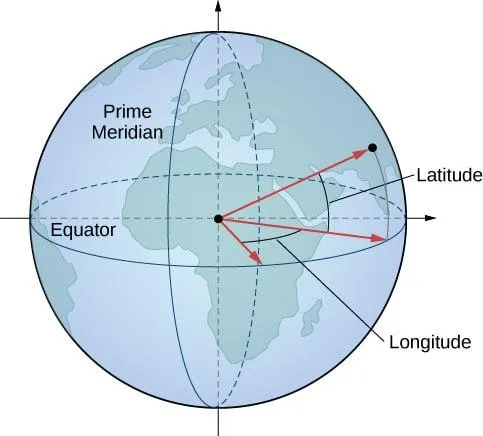
However, in most cases, it's not enough for us to just know where an object is located. We are interested in knowing how it interacts with other objects, and this is exactly what is taught in the school of drone pilots in the course Aerial Geodesy. To do this, we need to measure distances, lengths, areas, directions, etc.
Spherical coordinates are not well suited for measurements. The main reason is that an angular distance of 1 degree at different latitudes corresponds to a different linear distance on the Earth's surface: if 1 degree at the equator (or any other great circle line) is ≈111 km, then at latitudes other than 0 degrees this value will be less. In other words, the distance on the Earth's surface corresponding to 1 degree of angular distance is, generally speaking, a variable value that depends on the value of latitude. The use of rectangular coordinate systems frees us from such problems. Physically, the process of creating projections can be likened to projecting the rays of a light source from the center of a spheroid onto the projection surface (Fig. 6).
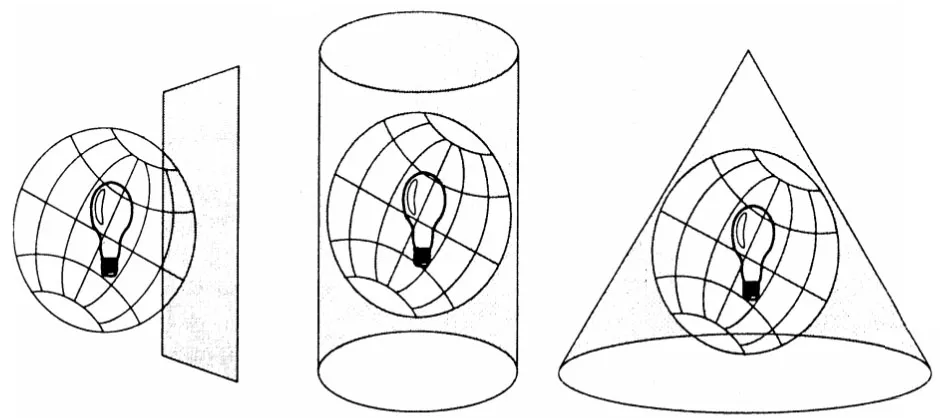
The shape to be designed is chosen so that it can be turned into a plane without stretching its surfaces. Common examples of shapes that meet this criterion are cones, cylinders, and planes. Depending on the choice of shape for projection, there are 3 families of map projections: conical, cylindrical, and planar.
The first step in creating a projection of one surface onto another is to create one or more points of contact. Each such point is called a point of contact. A plane projection is tangent to the globe at only one point. Tangent cones and cylinders make contact with the globe along the line. If the surface of the projection intersects the globe instead of simply touching its surface, the resulting projection conceptually requires the calculation of a line of sight rather than a tangent line. Regardless of whether the contact is a tangent or a line, its location is very important because it defines the point or lines of zero distortion. This line of true scale is often referred to as the standard line. In general, distortion increases with distance from the point of contact.
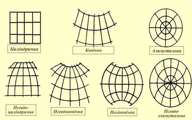
Projections are not absolutely accurate representations of geographic space. Each creates its own set of types and amounts of distortion on the map. There are distortions of shape (or angles), area, distance, and direction. Different types of map projections are used to represent different parts of the earth's surface. Some map projections minimize distortion in one parameter by increasing distortion in other parameters, while other projections try to minimize all distortions equally.
Figure 7 shows some types of projections. In general, there are hundreds of types and varieties of projections. But for us, cylindrical projections will be interesting, since they are used in drone navigation, and the Gauss-Kruger projection is just a transverse cylindrical projection.
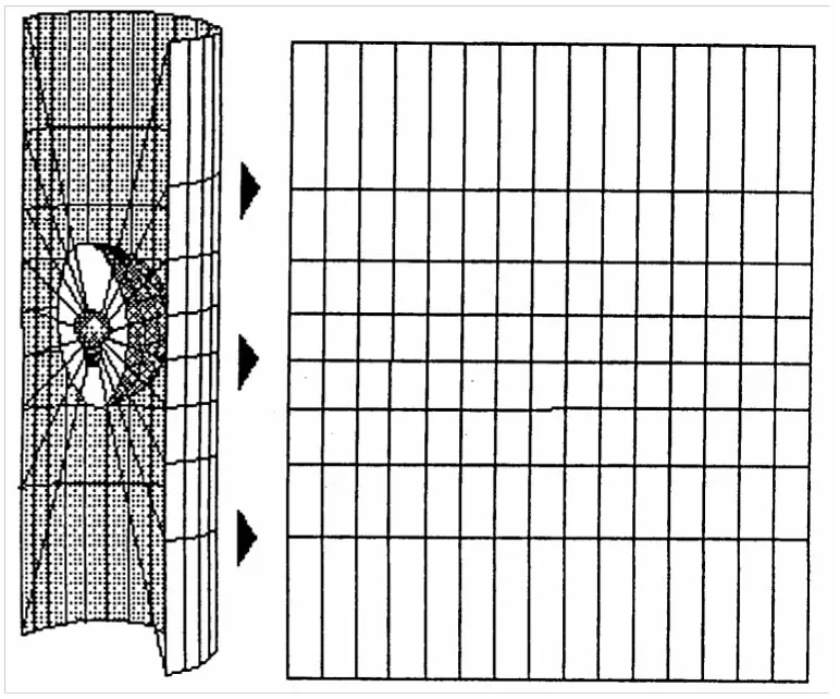
Cylindrical projections can have one line of contact or two lines of intersection on the globe. The equator is usually the line of contact. Meridians are projected geometrically onto the cylindrical surface, and parallels are projected mathematically to create 90° angles of the coordinate grid. The cylinder can be "bisected" along a meridian to obtain the final cylindrical projection (Figure 8). The meridians are spaced at regular intervals, while the interval between the parallel lines of latitude increases toward the poles.
This projection is equirectangular and shows the true direction along straight lines.
To create more complex cylindrical projections, the cylinder is rotated, thus changing the lines of contact or intersection. Transverse cylindrical projections, such as the Mercator or Gauss-Kruger transverse projection, use the meridians as lines of contact, so that the axis of the cylinder lies in the plane of the equator. The lines of contact go north and south, and the scale is true along them.
Now that the main stages of obtaining map projections have been considered and the characteristics of maps necessary for their understanding have been determined, we can give a detailed description of the SK-42 coordinate system.
5. SK-42.
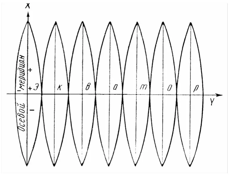
SK-42 can be characterized as rectangular coordinates in a zonal system. The zonal system in this case means the Gauss-Kruger projection. It divides the Earth's surface into 60 numbered zones of 6 degrees of width and 6 degrees of longitude each (Fig. 9).
The values of the extreme meridians of the six-degree zones will be as follows: the first zone 0 - 6 °, the second zone 6 - 12 °, the third zone 12 - 18 °, etc. It should be noted at once that the position of the zones in the Gauss-Kruger projection coincides with the position of the zones of the international system of dividing the earth's surface into six-degree zones (Fig. 10), called (by international agreement) columns, but differs in number. Since the numbering of the columns does not start from 0 ° meridian, but from 180 °, the zone number will differ from the column number by 30, that is:
n = N-30,
where n is the number of the six-degree coordinate zone, and N is the number of the column of the map sheets at a scale of 1: 1 000 000.
The CIS territory is located in zones 4 through 32. The zone number can be used to determine the longitude of the axial and extreme bordering meridians. For example, in zone 4, the westernmost meridian is 18°, the easternmost meridian is 24°, and the axial meridian is 21°.
Zonal projection implies that the projection is not performed simultaneously for the entire spheroid, but separately for each zone. The projection is performed as many times as there are zones. To obtain a projection of any of the 60 zones, the cylinder is placed relative to the spheroid in such a way that the surface of the cylinder is most closely adjacent to the surface of the spheroid within that zone. This method of projection minimizes the distortions that are inevitable during projection. The Gauss-Kruger projection is conformal (equirectangular), distortions of areas, distances and directions within each zone are minimal: there are no distortions along the axial meridian, therefore, the scale factor along the axial meridian is preserved and equal to 1. When moving away from the axial meridian, the distortion becomes different from 0 and reaches its maximum value of 1/750 at the zone boundary.
Latitude runs from pole to pole. Meridians and parallels are curved lines, except for the axial meridian. As mentioned above, each zone represents a specific coordinate system. The origin of each zone is located at the point where the equator intersects the zone's centerline. The coordinate system is rectangular. Each zone has its own origin. The axial meridian and the equator are taken as coordinate axes (Fig. 11): the axial meridian as the abscissa axis and the equator as the ordinate axis.
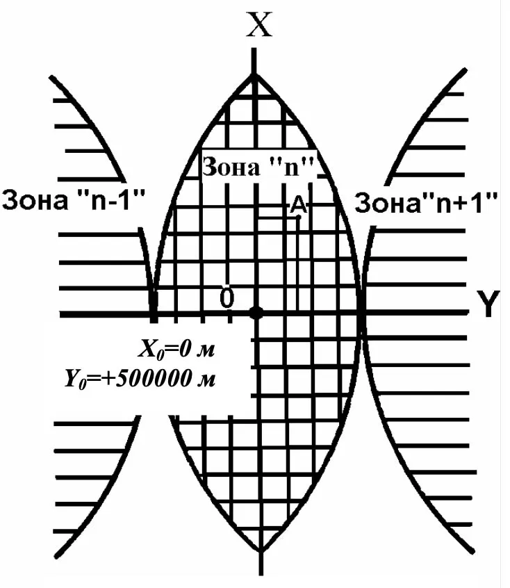
The unit of measurement is the meter. If the meridian is divided into equal segments and verticals are drawn through the dividing points, and small circles are drawn on the earth's surface at the same distances from each other and all this is projected onto a plane, observing the condition of equilateralism, then a grid of almost equal squares will appear on the plane. The lines that form the sides of these squares are called kilometer lines and are usually drawn on maps at a distance of several kilometers from each other. The lines of one system are parallel to the zone's midpoint, and the lines of the other system are parallel to the equator. Kilometer lines are drawn on all topographic maps and are used to determine the rectangular coordinates of points and to solve other map tasks.
The entire territory of the former USSR is located in the northern hemisphere, so the abscissa of all its points will be positive.
In order not to deal with negative coordinates, the ordinate of point 0, i.e. the origin, is conditionally accepted as 500 km (Fig. 11), or, alternatively, the value of the ordinates is increased by 500 km. Under these conditions, even at the equator, the westernmost point of the zone will have an ordinate of approximately +165 km. This technique is common and is used to define many coordinate systems (e.g., UTM). This shift is called is called a false eastward shift. Let's assume that two points are defined by their coordinates:
xA = 5,973 km, UA = 722 km, and xB = 5,973 km, yB = 395 km.
This means that the distance to both points from the equator is 5973 km and that point A lies in the zone east of the axial meridian at a distance of 222 km, and point B to the west - 105 km. The territory of the CIS is located in 28 zones. Thus, there will be 28 points with such coordinates within our country. To specify exactly which of the 28 points you are talking about, you must also specify the zone number, for example, 7. Enter the zone number and the ordinate. The ordinate will be: ya = 7722; yB = 7395. If y = 13,642, it means that the point is located in the 13th zone, and its conditional (increased by 500 km) ordinate is 642 km. As mentioned above, every topographic map has kilometer squares (on maps with a scale of 1:100,000, two kilometers), and the kilometer lines are labeled with integer numbers of kilometers from the corresponding axes.
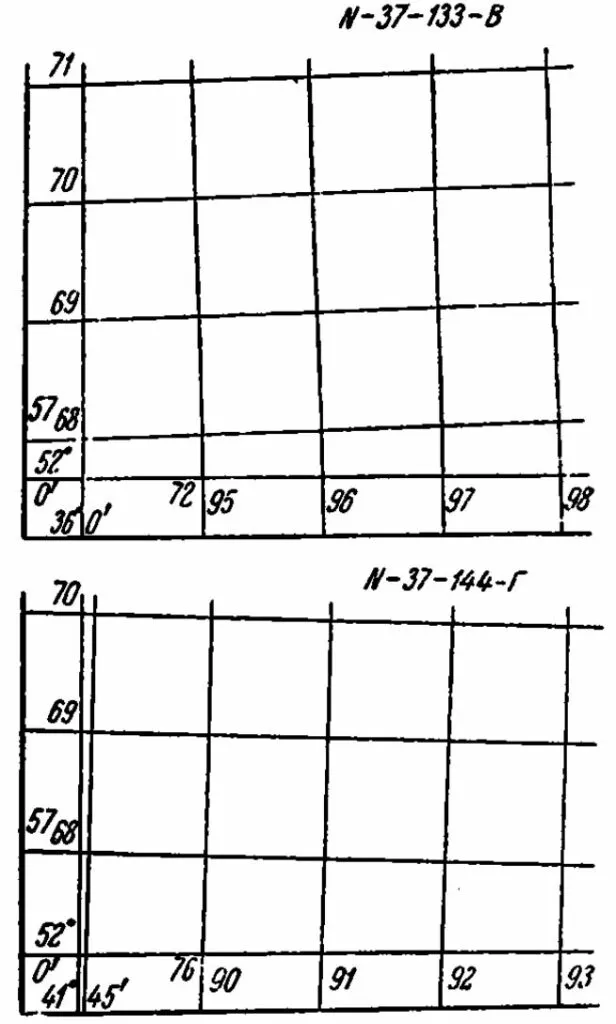
The kilometer diagrams for sheets N-37-133-B and N-37-144-G at a scale of 1:50,000 are shown in Figure 12.
The southernmost line on the map, perpendicular to the axial meridian, is labeled with the number of kilometers to this line from the equator along the axial meridian-5768. Other parallel lines, drawn through 1 km, are signed with the number of tens and units of kilometers, i.e. 69, 70, 71, etc. The first two digits of the abscissa value are not repeated, but only the last two digits are written. The abscissa is fully signed only in the upper and lower corners of the trapezoid.
Also, only the ordinates of the extreme lines are fully signed, such as 7295 on sheet K-37-133-B and 7690 on sheet K-37-144-G. The rest of the ordinates retain only the last two digits, respectively, 96, 97, 98, etc. And 91, 92, etc. The first digit in the ordinate, 7, indicates the zone number.
6. SK-42 and other geo-referencing issues.
When we deal with electronic maps or use remote sensing data in our work, it is almost always necessary to georeference them. Although this process is not complicated in itself, there are pitfalls to be aware of. As long as the working materials remain within the same coordinate system or projection, for example, SK-42, everything is simple. But when you move to data of a different scale, change the projection, combine data from different sources in one project, or move from local coordinates to global coordinates, these problems become apparent: images of objects in some layers are offset relative to the same objects in other layers. This can be caused by both objective circumstances and user errors.
Most GIS users who do not have a geodetic background believe that the width and length of any point on the Earth's surface are absolute values that do not depend on anything. Unfortunately, this is not the case. If you specify the same Geographic projection (Lat/Lon) for the input data and the result, but different ellipsoids (for example, Krasovsky and WGS-84), you will see that the latitude and longitude values of the same point on the two ellipsoids will be different. So, in order to reduce all data to one coordinate system or projection, you need to know all the parameters of the input and output projection absolutely accurately. It should be remembered that the process of projecting and re-projecting the original data is a rather cumbersome recalculation, which can result in errors. These errors are caused by computer rounding errors and shortcomings of computational algorithms.
A problem often arises when the study area crosses two or more zones, because geographical boundaries often do not correspond to the structure of the zones. If your study area spans more than one zone, you have several options to choose from.
For example:
- Determine which zone occupies most of the study area (for example, zone 9). Then include the remaining area outside this zone in the coordinate system of zone 9. This approach can have an unexpected effect because you are using the standard parallels of zone 9 to project another zone. As a result, the objects of the other zone may be distorted (in other words, shifted) by several hundred meters.
- Discard the SK-42; choose another projection. Perhaps your new projection and coordinate system will avoid these problems.
- Create your own projection. It may suit you at the moment, but problems may arise later because no one will know which projection you used. Problems can arise because you may unknowingly give or receive data in different coordinate systems.
- Store everything in decimal degrees and project when the need arises.
Translating a map or image from one projection to another is usually done in two or three steps. At the first step, the coordinates of the original projection are converted to geographic coordinates - latitude and longitude. That is, the inverse projection problem is solved. If the source and target projections use the same reference - an ellipsoid, then the second step is to convert the obtained geographic coordinates to the coordinates of the target projection, that is, a simple direct projection. It is very simple: from one projection to the ellipsoid, and then to another projection. ESRI and ERDAS software can perform direct projection on the fly when displaying and analyzing data. Therefore, it is obvious that it often makes sense to store data not in flat projection coordinates (kilometer), but in angular geographic coordinates. In this case, when changing the projection, the first step - reverse projection - will not be performed, which inevitably reduces the accuracy of the data due to the limited accuracy of the representation of numbers in the computer and rounding errors in calculations (often the main factor is the representation of the reverse projection using polynomials due to the inability to obtain an exact formula). On the other hand, on-the-fly projection requires performing the appropriate calculations, which, of course, reduces the display speed. but if it is known for certain that the projection will not change, then it makes sense to store and project the data. If it is possible to store and project non-projected data as well, it is better to use it. If the source and target projections use different reference ellipsoids or geodetic dates, the second step is to recalculate the horizontal geographic coordinates from one ellipsoid to another, and the conversion to the target projection is the third step.
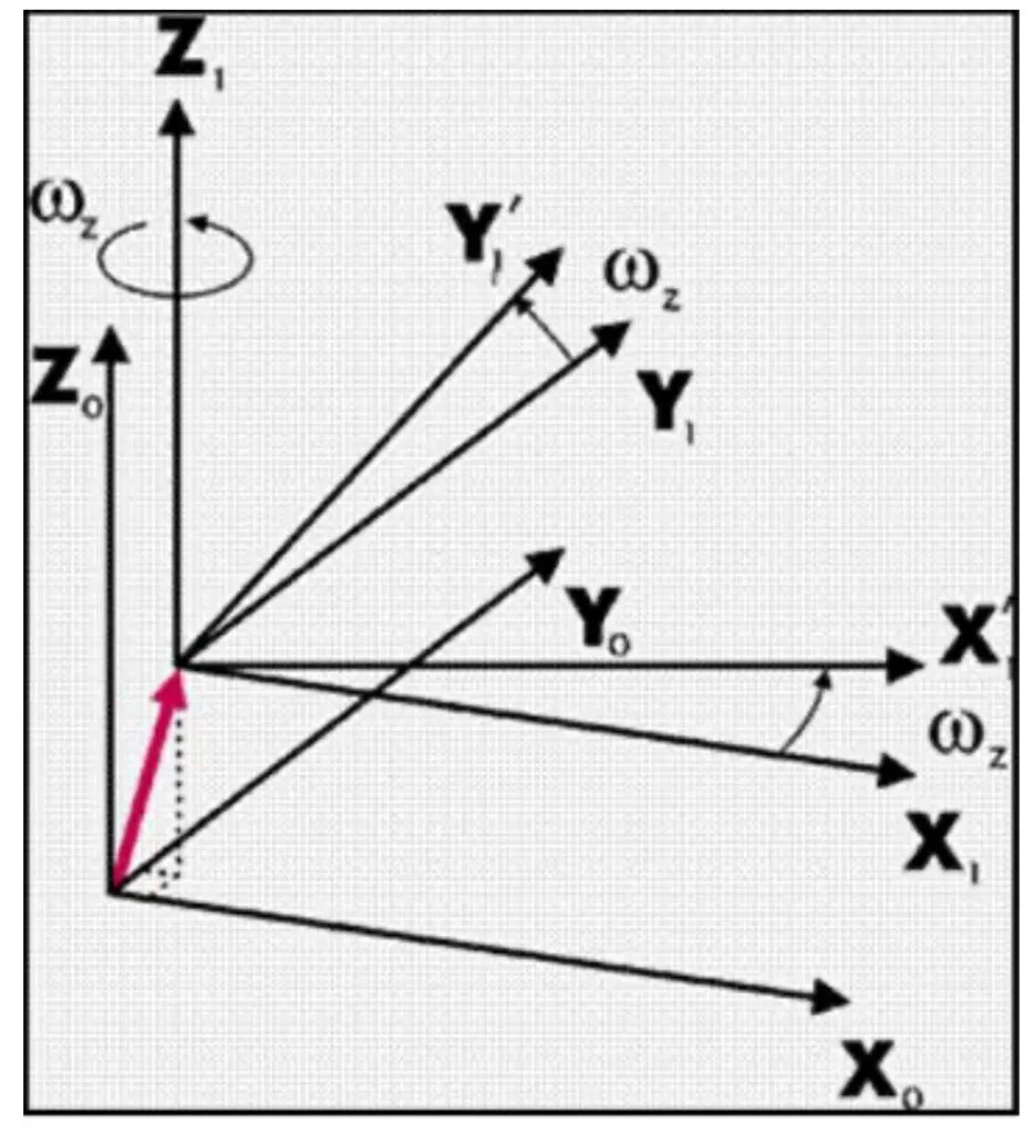
From the ellipsoidal coordinates, it is easy to move to a three-dimensional rectangular coordinate system with the origin in the center of the ellipsoid (geocentric coordinate system), then the transition from one ellipsoid to another will be determined by the relationship of the geocentric coordinate systems of these two ellipsoids (Figure 13). In general, such a relationship can be expressed by seven linkage parameters - shifts of the origin along each axis (three linear parameters), rotations around each axis (three angular parameters), and one scaling factor. In general, this transformation is performed using Helmert's formulas. Since rotation and scaling are not always necessary, a simpler three-parameter transformation is sometimes used. In some cases, more complex multivariate regression equations are used to transform ellipsoids.
When using different ellipsoids, it should be borne in mind that not all combinations of ellipsoids have accurate and unambiguous coupling parameters at present. For example, the coupling parameters of SK-42 and PZ-90 are known exactly. At the same time, there are several variants of the coupling parameters of the PZ-90 and WGS-84. Moreover, the displacement of objects on the Earth's surface when using different variants can reach hundreds of meters, which is unacceptable for a large scale. Until the official values of the communication parameters are published, the solution to this problem can be to use only one known option. When purchasing data from different sources, it is necessary to obtain along with them the communication parameters used to switch from SK-42 to WGS-84, if such a conversion took place. It is these communication parameters that must be incorporated into the software to obtain correct results.
To study at the quadcopter drone pilot school, we recommend that you do some independent work:
Determine the parameters of the cartographic coordinate system SK-42 in relation to the territory of Ukraine:
Type of projection and its name -
Zone number -
Spheroid-scale factor-central meridian-latitude of reference-
False eastward shift -
False northward shift -
Coordinate units -
Distance units -